Tag Archives: LiDAR

How OCAD Helps you With Positioning and Mapping in the Field

In this blog post, we’ll show you the tools OCAD offers for adding great base data to your mapping project—tools that help you determine your location in the field and allow you to identify and map terrain features, vegetation, and man-made objects.

As you’ll see at the end of this article, all of this base data can be used in the OCAD App to map efficiently and accurately.

LiDAR

If you have access to up-to-date LiDAR data, consider yourself lucky. With LiDAR data, you can create excellent base maps that not only allow you to pinpoint your location but also help you identify many map features.


OCAD calculates two types of Contour Lines: smoothed (green) and not-smoothed (blue). Use the not smoothed contour lines as a background during field mapping, which includes all the details. To draw contour lines on the PC, you can start with the smoothed contours and adjust them as needed using the Reshape function.

Smoothed (green) and not-smoothed (blue) contour lines.

The Hill Shading Map reveals numerous terrain features that are not visible in the contour lines, such as roads, forestry tracks, gullies, small pits and knolls.

Hill shading map of same map extent as above.

The Feature Map is similar to the Hill Shading Map, but also shows features that are close to the ground such as stones, walls, tree trunks, fences, or cars which were previously not or only poorly recognizable on background maps.

Feature map of same map extent as above.

The Las Intensity Map helps you to distinguish between deciduous and coniferous trees.

Intensity map of same map extent as above.

The Vegetation Height Map shows vegetation features ranging from open areas (yellow) and ground vegetation (red) to dense vegetation (green), open forest (white) and high trees (blue). The latter can be particularly useful in open forest with few ground vegetation.

Vegetation height map of same map extent as above.

The Vegetation Base Map is similar to the Vegetation Height Map but focus more on the runabilty of the terrain.

Vegetation base map of same map extent as above.

GPS

GPS is another key tool for determining position, especially when there is no or insufficient Lidar data available.

If your mobile device does not have a built-in GPS module, or if the built-in module is not accurate enough, you can connect it to an external GPS receiver.

In the OCAD App, you can use GPS not only to determine your location, but also to directly capture sketches and objects

We recently published a comprehensive article titled GPS in Orienteering Map Map Making that provides information about GPS and its use with OCAD.

GPS track and GPS position in urban area.

Cadastral maps

Detailed cadastral maps are particularly useful for sprint maps, and they often allow you to pinpoint your exact location and map many features such as buildings, roads or boundaries.

You can import cadastral maps into OCAD in various formats (Shape, GeoPackage, DXF) or load them as a WMS/WMTS background map.

Cadastral map of same map extent as above.

Areal images / Orthophotos

In open terrain, aerial photos and orthophotos can help with positioning and recognizing objects that are not visible on cadastral maps.

You have the following options for loading a georeferenced aerial photo into OCAD.

Aerial image of same map extent as above.

Using the Background Maps and Tools in the OCAD App

Head out into the field with the best possible base map!

All of this base data can be used in the OCAD App to map efficiently and accurately. In the app, you can show or hide various base maps or symbols and show your current GPS position.

  • You can easily show, hide or change the opacity of base maps in the Layers Panel.

  • You can turn GPS on or off in the Positioning settings.

  • You can also easily show or hide symbols (e.g. hide unsmoothed contour lines)

Feature Map – Get more out of your LiDAR Data

In the latest OCAD Update, the option Create Feature Map was added to the DEM Wizard to gain even more information from LiDAR data.

The Feature Map can be used to recognize objects close to the ground such as stones, walls, tree trunks, fences, or cars which were previously not or only poorly recognizable on background maps that can be created with the DEM Wizard in OCAD.

How the creation of Feature Maps works

In a LiDAR file, each point is typically assigned to a class based on the reflection of the laser pulse, such as ground, vegetation, buildings or water. Only ground points are used to generate the Hill Shading and Slope Gradient map. This means that a lot of information is lost that is available in points classified differently.

To generate the Feature Map, OCAD reclassifies the LiDAR points so that not only ground points but all points are used for the calculation. You can further define from and up to which height points are taken into account.

Example stone detection
Pontresina, Switzerland
LiDAR data from 2022, 29 points per square meter, 0.5m cell size, 0.0-2.0m threshold.

Orienteering Map of stony terrain.
Slope Gradient Map. Most stones are not visible. The stones that are visible are probably overgrown and therefore classified as ground points.
Feature Map. Some stones becomes clearly visible.

Example stone wall detection
Jura, Switzerland
LiDAR data from 2020, 25 points per square meter, 0.5m cell size, 0.0-1.5m threshold.

Slope Gradient Map. The stone walls are only partially visible.
Feature Map. The stone walls become clearly visible.

Example tree trunks detection
S-chanf, Switzerland
LiDAR data from 2022, 25 points per square meter, 0.5m cell size, 0.0-0.5m threshold.

Slope Gradient Map.
Feature Map. Tree trunks are visible and can help to determine the exact position.

Example urban area
Zeiningen, Switzerland
LiDAR data from 2020, 13 points per square meter, 0.5m cell size, 0.0-2.0m threshold.

Slope Gradient Map.
Feature Map. Hedges, walls, cars and bridges becomes visible.
Vegetation Height Map. Most of the objects on the Feature Map are also visible on this map.

Example without satisfactory result
Lillehammer, Norway
LiDAR data from 2017, 10 points per square meter, 0.75m cell size, 0.0-2.0m threshold.

Slope Gradient Map.
Feature Map. In this area there are many small trees and bushes with branches down to the ground. It is difficult to distinguish, for example, large stones from trees or knolls from this data.
Vegetation Height Map of the same area.

Conclusion:

The information content of the feature map depends on the terrain type, the settings you choose in the dialog and the quality of the LiDAR data, in particular the point density. With good data quality, the feature map can be a useful addition to the existing background maps, to detect objects and help the cartographer to determine the exact position in the terrain.

Credit goes to Jeff Teutsch and his Lidar Case Study – Using simple ground reclassification to see features in data.

MapAnt Switzerland

After the release of a pilot project for a Swiss MapAnt last summer, we are happy to present our final MapAnt Switzerland, which covers the whole of Switzerland.

The creation of this map became possible after the Federal Office of Topography swisstopo made many of its data available online free of charge as Open Government Data (OGD) this March.

MapAnt can animate to discover new areas. However, please note, that the possession of this map does not entitle to any orienteering activities in the terrain. Before using this map in the terrain, it is mandatory to contact the local orienteering club or the regional orienteering association to clarify forest use, private property, nature reserves, wildlife reserves, protected areas and other restrictions.

You can find more information about the development of MapAnt in our OCAD Wiki.

Have fun exploring Switzerland digitally!

Multi-directional Hillshading

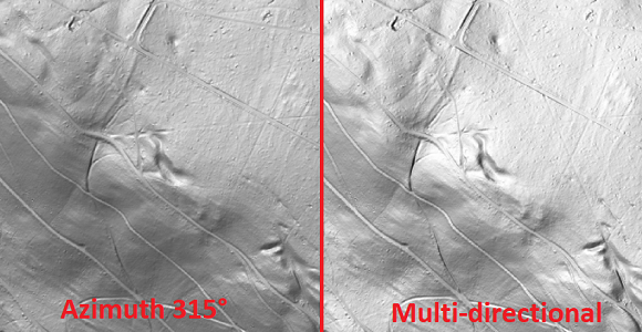
A hillshade is a shaded relief picture of the surface. Important for a hillshade is the position of the imaginary light source, which is taken into account for shading the image.

Normally, the direction of the light source is 315° (north-west). Since the Service Update 20.5.3, it’s also possible to choose the option Multi-directional. It is a composite image made up of four images in which the light source comes from different directions. Like this, the terrain is more realistically represented, and overexposed and nonilluminated areas of the map are more balanced.

In OCAD, Hill Shading can be created from the DEM menu or from the DEM Import Wizard.

How to use OCAD and LiDAR to Calculate Climbing for Courses

In order to indicate the climbing for courses, many course setters invest a lot of time to manually add up the climbing along the optimal route. If a terrain model (DEM) is available, this can be done easier with OCAD. With the following workflow, which is also possible in the OCAD Course Setting Edition, the climbing can be calculated automatically to a certain extent:

  1. Start a course setting project, open a background map and draw a course.

2. In your course setting project, go to menu DEM > Open and open your terrain model (* _DTM.ocdDem). This file is generated during the LiDAR processing.

3. Now draw a line with the optimal route from start to finish. This has to be done for each course. Use any line symbol in the symbol box or create a new one.

4. Select one of these optimal routes and go to menu DEM > Create Profile. You will get a Total ascent value, which you can enter into Course Setting > Courses > Climb used.

In the Courses dialogue, there is also a Climb calculated value, which is just calculated automatically by adding the net ascent from each control to the next one. The value that is entered in Climb used will show up in the control description.