DHM

A DEM (Digital Elevation Model) contains points with elevation data. DEM Data are based on LIDAR (Light Detection and Ranging) technology measurement, also known as Airborne Laser Scanning. There are DEM with point data arranged in a regular grid with a constant distance between the points. This distance is called cell size. Other DEM contain data points arranged irregularly (cloud-model).

Read more about this topic: http://en.wikipedia.org/wiki/Digital_elevation_model

Import

The OCAD DEM Module is able to import files with regular and irregular DEM data. Supported DEM data formats are: ESRI ASCII Grid (*.asc), Raw data ASCII XYZ file (*.xyz), ASCII Grid XYZ file (*.xyz), LAS file (*.las) and SRTM file (*.hgt) file.

1. Open a map or create a new one.
2. Select Import from the DEM menu. First use Add button to add at least 1 DEM to the DEM Import dialog.
3. Analyze the DEM to get some information about the DEM like extent, cell size etc.
4. If the source file is a regular grid (data type of import files = grid), the Cell size box is set to read only. OCAD sets the same cell size for the imported DEM. For irregular DEM data source (data type of import files = raw) the cell size can be set in the 'cell size' box. For these DEM's OCAD interpolates a regular grid with the specified cell size during the import.
5. At the end of the import procedure the imported DEM must be saved in the OCAD DEM file format (*.ocdDem) and it is loaded to the OCAD map.
6. To see the extent of the loaded DEM activate the Show Frame menu item.

The Cell size range is between 0.01 and 650 m.
For DEM's with negative elevation values use the option Do not save negative height values to set them to 0.
DEM import is limited to approximately 25 mio. data points, resp. 20 mio. data points for LAS files.

LAS data import:

• Choose ground classification and Last return option to create a terrain model from LAS data.
• Choose all classifications and First return option to create a surface model from LAS data.

During LAS data import a classification image and a intensity image are created and loaded as background maps. A difference image between the first and last return is created if the All returns option in the DEM Import dialog is choosen.
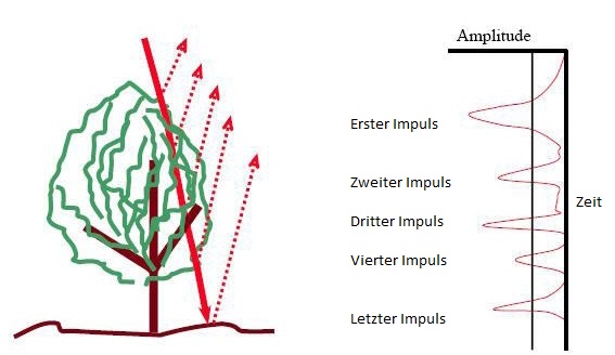
A Radar beam splits as it hits objects. The result are multiple returns. LIDAR can collect up to four returns. The difference between first and last return can show object height. The last return doesn’t always reach the ground.

Source: Lohani, Bharat. Airborne Altimetric LiDAR: Principle, Data Collection, Processing and Applications.

SRTM hgt data import:

• This is a world wide available DEM data set from the Shuttle Radar Topography Mission (SRTM).
• The data files and documentation: [1]

SRTM hgt data import requires that a coordinate system set in the OCAD map file.

Open

Open an OCAD DEM file (*ocdDem).

Show Frame

Shows blue rectangle with the extent of the loaded DEM.

Resize

Resize the loaded OCAD DEM file (make a subset) and save it as a new OCAD DEM file.

Info

Shows information about OCAD DEM file.

When moving the mouse cursor over the file name then the file name with path appears.

Close

Close OCAD DEM file.

Merge DEM

Choose Merge from DEM menu to merge two different DEMs.

• DEM 1: Choose the first DEM.
• DEM 2: Choose the second DEM.

The two DEMs must have the same cell size and image clipping.

Calculate DEM Difference

1. Choose Calculate DEM Difference from DEM menu.
2. The Calculate DEM Difference dialog box appears.
3. Add Upper DEM = DSM data file
4. Add Lower DEM = DEM data file
5. Click OK.

To visualize the DEM difference choose [Classify Vegetation Height]

• No difference between the elevation models appears black.
• The greater the difference, the whiter it appears.

Same data format, cell size and clipping of DSM and DEM required.

Create Contour Lines

This function calculates contour lines based on the loaded DEM.

• Define 1-3 contour intervals (for example 1m, 5m, 25m) and a pre-selected line symbol (according to the first three line symbols in the settings) for each type appears (can be changed).

Contour interval values can be entered manually or chosen from the list.

• Specify the minimum (lowest) and maximum (highest) contour for the calculation.

Create Hypsometric Map

This function calculates a grayscale or colored hypsometric map as GeoTIFF file.

Optionally it is directly loaded as background map.

Two different types of hypsometric maps can be edited:

• Grayscale hypsometric map
• Colored hypsometric map

Create Hill Shading

This function calculates a shaded relief picture (hill shading).

There are two calculation methods available:

• Slope shading is optimized to see outlines of features like paths in a slope.
• Slope shading combined with oblique light shading is the recommended method if the hill shading should be used as a background relief of a map. Optionally the calculated hill shading is directly loaded as background map.

Aside from the chosen method an Azimuth and a Declination of the light source has to be set. Standard settings are 315° (north-west) and 45°. An Exaggeration factor of 4 is pre-selected and can be altered.

Calculate Slope Gradient

Choose Calculate Slope Gradient from DEM menu.

The Calculate Slope Gradient dialog box appears.

Select one of two different methods:

• Continous (<x° = grayscale / >x° = black)
• Black/White (<x° = white / >x° = black)

The resulting picture can be used to identify cliffs an rock faces. The result can sometimes be significantly improved with a slight adjustment of the gradient (between 42-45 degrees).

Slope gradient also shows paths or relief features independent from a azimut like the Hill Shading.

Classify Vegetation Height

Choose Classify Vegetation Height from DEM menu.

There are two different options to show vegetation height classification:

• Gray scale classification with options: Linear, Quadratic negative, Quadratic positive
• Colored classification: Define classes with a height and color range

- Split a class into two classes by clicking the Split class button

- Remove a class by clicking the Remove class button

- Load the settings from a text file by clicking the Load button

- Save the settings to a text file by clicking the Save button

- Reset the classes and colors to the default settings by clicking the Reset classes to default button

Create Profile

To create a profile:

1. Select a line object within the DEM data.
2. Choose the Create Profile command from the DEM menu.
3. The DEM Profile dialog appears and the profile is shown. You have several options now:

• Auto scale: If this option is enabled, OCAD takes a scale which fits best to the dialog box.
• Scale: Choose the desired scale of the profile in the dropdown list.
• Show grid: If this box is activated, a grid is shown in the profile.
• Elevation factor: Choose an elevation factor in the dropdown list. This is the scale factor for the horizontal profile axis (height).
• The Elevation resolution and the Length resolution are filters that influence the calculation of the total ascent and total descent. These resolution values should not be more accurate than the elevation resolution and cell size of the DEM.

DEM Profile dialog is a non-modal dialog. The user can switch to the OCAD map window. It is possible to edit the selected line object in the OCAD map. Click the Update button in the DEM Profile dialog to see the profile for the edited or newly selected object.

Export Profile

Export OCD
Click the Export OCD button to export the profile to a new OCD-File. The DEM Profile Options dialog appears.

The Template DEM Profile.ocd file in the OCAD-directory is chosen as a template file (for the symbol set, colors etc.) by default. You can choose an own template by clicking the Load template button.

In the Units and Formats category, you can choose, wheter the distance is to be shown in km or in m. In addition, you can set the time format (at the moment only h:mm is available) and the rounding (no rounding, 5 minutes, 10 minutes). Uncheck the Show text at the bottom of the profile option if you do not want any text under the profile.

In the Labels and Symbols category, labels and symbols can be allocated to the start- and endpoint or a stopover. Enter a label in the corresponding field (for example the name of a place) and choose a symbol from the dropdown list. These symbols are defined in the template file.

Click the OK button when finished. In the next dialog you have to save the profile at the desired location. To open the document, use the Open Recently Exported Documents function in the File menu. The profile can be edited (e.g. change colors or add objects) there.

Export BMP/GIF Click the Export BMP/GIF button to export the profile as a raster image. The Save Picture dialog box appears. Browse a location and enter a name for the new file. Choose the file type in the Save as type drop down list. Click the Save button to finish. The profile

Add to map

Print

Export

Export OCAD DEM file as ESRI ASCII Grid or as ASCII Grid XYZ. Select Create tiles for large DEMs.

Previous Chapter: Printing Maps

Next Chapter: GPS

Back to Main Page